Editor guide

Md-math-field is made with carta-md and mathlive (so if you want, you can go straight to the source docs). It supports:

markdown
katex math
tikzjax with these tikz packages:
- chemfig
- tikz-cd
- circuitikz
- pgfplots
- array
- amsmath
  - amstext
- amsfonts
- amssymb
- tikz-3dplot

Latex examples

alt text

Formula is small $\frac{x^2+23x}{\int_2^3 3 dx}$\
Formula is big $\displaystyle \frac{x^2+23x}{\int_2^3 3 dx}$\
Formula is big and centered
$$
\frac{x^2+23x}{\int_2^3 3 dx}
$$

alt text

Question text with a number $123$ or decimal with no spaces $0{,}123$, then newline

and then additional newline

\
TAB |&emsp;| and SPACE additional |&ensp;| and can be put together | &emsp; &emsp; &emsp; |... like that...

And then the number 
1. is the same as 
1) and makes a list when in new line. But can be escaped with \ like this:

1\), 2\), 3\)... For measurements in text we use basic cm², cm³ symbols. And yet another symbol - endash (lithuanian dash): – And that's it...

alt text

Closed question with choices...

**A** Choice $1$ &emsp;
**B** Choice $2$ &emsp;
**C** Choice $3$ &emsp;
**D** Choice $4$

Useful tikz examples (math templates)

alt text

```tikz
\begin{document}
\begin{tikzpicture}[scale=1.5]

	\coordinate (A) at (-2,-1);
	\coordinate (B) at (-2,1);
	\coordinate (C) at (2,1);
	\coordinate (D) at (2,-1);
	
	\draw (A) -- (B) -- (C) -- (D) -- (A) -- (C);
	\draw (B) -- (D);
	
	\node[left, scale=1.5] at (A) {$A$};
	\node[left, scale=1.5] at (B) {$B$};
	\node[right, scale=1.5] at (C) {$C$};
	\node[right, scale=1.5] at (D) {$D$};
	\node[below, scale=1.5] at (0,0) {$O$};
	\node[below, scale=1.5] at (0,-1) {$x+4$};
	\node[left, scale=1.5] at (-2,0) {$x$};
	

\end{tikzpicture}
\end{document}
```

alt text

```tikz
\begin{document}
\begin{tikzpicture}

% Axis
\draw (-2,0) -- (2,0);
\fill (2,0) -- (1.8,0.1) -- (1.8,-0.1) -- cycle;
\node[below, scale=1.5] at (1.9,0) {$x$};

\coordinate (-B) at (-1.8,0);
\coordinate (B) at (-1,0);
\coordinate (BC) at (0,0);
\coordinate (C) at (1,0);
\coordinate (C+) at (1.7, 0);

\draw (B) circle (2pt);
\node[below, scale=1.5] at (B) {$0$};

\fill (C) circle (2pt);
\node[below, scale=1.5] at (C) {$\frac12$};

\node[above, scale=1.5] at (-B) {$-$};
\node[above, scale=1.5] at (BC) {$+$};
\node[above, scale=1.5] at (C+) {$-$};

\draw[thick] (B) arc[start angle=180, end angle=0, x radius=1, y radius=0.7];
\draw[thick] (C) arc[start angle=180, end angle=90, x radius=1, y radius=0.7];
\draw[thick] (B) arc[start angle=-360, end angle=-270, x radius=1, y radius=0.7];

\end{tikzpicture}
\end{document}
```

alt text

```tikz
\begin{document}
\begin{tikzpicture}

% Axis
\draw (-2,0) -- (2,0);
\fill (2,0) -- (1.8,0.1) -- (1.8,-0.1) -- cycle;
\node[below, scale=1.5] at (1.9,0) {$x$};

\coordinate (-B) at (-1.8,0);
\coordinate (B) at (-1,0);
\coordinate (BC) at (0,0);
\coordinate (C) at (1,0);
\coordinate (C+) at (1.7, 0);

\fill (B) circle (2pt);
\node[below, scale=1.5] at (-1.2,0) {$0$};

\draw (C) circle (2pt);
\node[below, scale=1.5] at (C) {$1$};

\node[above, scale=1.5] at (-B) {$+$};
\node[above, scale=1.5] at (BC) {$-$};
\node[above, scale=1.5] at (C+) {$+$};

\draw[thick, domain=-2:2, samples=100] plot (\x, {0.7*(\x+1)*(\x-1)});


\end{tikzpicture}
\end{document}
```

alt text

```tikz
\begin{document}
\begin{tikzpicture}

% Axis
\draw (-6,0) -- (2,0);
\fill (2,0) -- (1.8,0.1) -- (1.8,-0.1) -- cycle;
\node[below, scale=1.5] at (1.7,0) {$x$};

% Interval start point
\coordinate (-B) at (-6,0);
\coordinate (B) at (-4,0);
\coordinate (C) at (-2,0);
\coordinate (D) at (0,0);
\coordinate (D+) at (1.7, 0);

\draw (B) circle (1.5pt);
\node[below, scale=1.5] at (B) {$-4$};

\fill (C) circle (1.5pt);
\node[below, scale=1.5] at (C) {$-\frac12$};

\draw (D) circle (1.5pt);
\node[below, scale=1.5] at (D) {$\frac23$};

\foreach \x in {-6,-5.85,...,0} { 
	\draw (\x,0) -- (\x-0.5,0.4);
}

\foreach \x in {-4, -3.85,...,1.7} { 
	\draw (\x,0) -- (\x-0.5,-0.4);
}

\foreach \x in {-2, -1.85,...,1.7} { 
	\draw (\x,0) -- (\x+0.5,-0.4);
}

\end{tikzpicture}
\end{document}
```

alt text

```tikz
\usepackage{pgfplots}

\begin{document}

\begin{tikzpicture}
    \begin{axis}[
        axis lines=middle,
        xlabel={$x$},
        ylabel={$y$},
        samples=100,
        domain=0:9,
        ymin=0, ymax=5,
        xmin=-0.5, xmax=9,
        xtick={0,1},
        ytick={0,1,2},
		extra x ticks={0},
		extra x tick labels={$0$},
		extra x tick style={tick label style={font=\small}},
        tick label style={font=\small},
    	scale only axis,
	    width=7cm,
    	height=3cm
    ]
        \addplot[thick, violet] {sqrt(x) + 2};
    \end{axis}
\end{tikzpicture}

\end{document}
```

alt text

```tikz
\usepackage{pgfplots}

\begin{document}

\begin{tikzpicture}
    \begin{axis}[
        axis lines=middle,
        xlabel={$x$},
        ylabel={$y$},
        samples=100,
        domain=-4:4,
        ymin=-3, ymax=5,
        xmin=-4, xmax=4,
        xtick={0,2},
		ytick={0},
		extra x ticks={-0.2},
		extra x tick labels={$0$},
		extra x tick style={tick label style={font=\small}},
        tick label style={font=\small},
    	scale only axis,
	    width=5cm,
    	height=5cm
    ]
        \addplot[thick, violet] {x^2-2*x};
		\addplot[only marks, mark=*, mark size=1pt, black] coordinates {(2,0)};
		\addplot[only marks, mark=*, mark size=1pt, black] coordinates {(0,0)};

    \end{axis}
\end{tikzpicture}

\end{document}
```

alt text

```tikz
\begin{document}
\begin{tikzpicture}

% Axis
\draw (-4,0) -- (2,0);
\fill (2,0) -- (1.8,0.1) -- (1.8,-0.1) -- cycle;
\node[below, scale=1.5] at (1.9,0) {$x$};

\coordinate (-A) at (-3.7,0);
\coordinate (A) at (-3,0);
\coordinate (AB) at (-2,0);
\coordinate (B) at (-1,0);
\coordinate (BC) at (0,0);
\coordinate (C) at (1,0);
\coordinate (C+) at (1.7, 0);

\draw (A) circle (2pt);
\node[below, scale=1.5] at (A) {$0$};

\draw (B) circle (2pt);
\node[below, scale=1.5] at (B) {$1$};

\draw (C) circle (2pt);
\node[below, scale=1.5] at (C) {$3$};

\node[above, scale=1.5] at (-A) {$-$};
\node[above, scale=1.5] at (AB) {$+$};
\node[above, scale=1.5] at (BC) {$-$};
\node[above, scale=1.5] at (C+) {$+$};

\draw[thick] (A) arc[start angle=180, end angle=0, x radius=1, y radius=0.7];
\draw[thick] (B) arc[start angle=180, end angle=0, x radius=1, y radius=0.7];
\draw[thick] (C) arc[start angle=180, end angle=90, x radius=1, y radius=0.7];
\draw[thick] (A) arc[start angle=-360, end angle=-270, x radius=1, y radius=0.7];

\end{tikzpicture}
\end{document}
```

alt text

```tikz
\begin{document}
\begin{tikzpicture}

% Axis
\draw (-2,0) -- (2,0);
\fill (2,0) -- (1.8,0.1) -- (1.8,-0.1) -- cycle;
\node[below, scale=1.5] at (1.9,0) {$x$};

\coordinate (-B) at (-0.8,0);
\coordinate (B) at (0,0);
\coordinate (BC) at (0.8,0);

\draw (B) circle (2pt);
\node[below, scale=1.5] at (B) {$3$};

\node[above, scale=1.5] at (-B) {$-$};
\node[above, scale=1.5] at (BC) {$-$};

\draw[thick] (B) arc[start angle=180, end angle=90, x radius=1, y radius=0.7];
\draw[thick] (B) arc[start angle=-360, end angle=-270, x radius=1, y radius=0.7];

\end{tikzpicture}
\end{document}
```

More tikz examples

alt text

```tikz
\begin{document}
  \begin{tikzpicture}

  % Draw grid
  \draw[step=1cm,very thin,color=black!50] (-5,-5) grid (5,5);

  % Draw axes
  \draw[->] (-4.2,0) -- (4.2,0) node[below] {$x$};
  \draw[->] (0,-4.2) -- (0,4.2) node[right] {$y$};

  % Draw absolute value function
  \draw[thick,blue,domain=-4:4] plot (\x,{abs(\x)}) node[right] {$y = |x|$};

  % Draw horizontal line y=2
  \draw[thick,green!80!black] (-4,2) -- (4,2) node[right] {$y = 2$};

  % Labels for specific points
  \node[below] at (1,0) {1};
  \node[left] at (0,1) {1};

  \end{tikzpicture}
\end{document}
```

alt text

```tikz

\begin{document}
\begin{tikzpicture}

    % Draw grid
    \draw[step=1cm,very thin,color=black!50] (-5,-2) grid (5,6);

    % Draw axes
    \draw[->] (-4.2,0) -- (4.2,0) node[below] {$x$};
    \draw[->] (0,-2.1) -- (0,5.2) node[right] {$y$};

    % Draw absolute value function
    \draw[thick,blue,domain=-2.5:2.5] plot (\x,{pow(\x, 2)}) node[right] {$y = x^2$};

    % Labels for specific points
    \node[below] at (1,0) {1};
    \node[left] at (0,1) {1};

\end{tikzpicture}
\end{document}

```

alt text

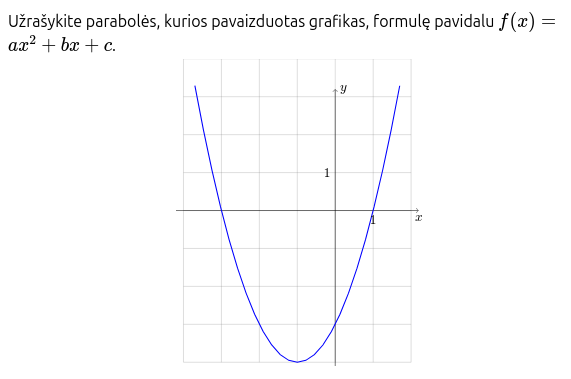
Užrašykite parabolės, kurios pavaizduotas grafikas, formulę
pavidalu $f(x) = ax^2 + bx + c$.

```tikz
\begin{document}
  \begin{tikzpicture}

    % Draw grid
    \draw[step=1cm,very thin,color=black!50] (-4,-4) grid (2,4);

    % Draw axes
    \draw[->] (-4.2,0) -- (2.2,0) node[below] {$x$};
    \draw[->] (0,-4.1) -- (0,3.2) node[right] {$y$};

    % Draw absolute value function
    \draw[thick,blue,domain=-3.7:1.7] plot (\x,{pow(\x, 2) + 2 * \x - 3});

    % Labels for specific points
    \node[below] at (1,0) {1};
	\node[left] at (0,1) {1};

  \end{tikzpicture}
\end{document}
```

Generic tikz examples

Official tikz examples

alt text

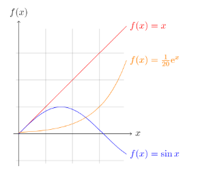
```tikz
\begin{document}
  \begin{tikzpicture}[domain=0:4]
    \draw[very thin,color=gray] (-0.1,-1.1) grid (3.9,3.9);
    \draw[->] (-0.2,0) -- (4.2,0) node[right] {$x$};
    \draw[->] (0,-1.2) -- (0,4.2) node[above] {$f(x)$};
    \draw[color=red]    plot (\x,\x)             node[right] {$f(x) =x$};
    \draw[color=blue]   plot (\x,{sin(\x r)})    node[right] {$f(x) = \sin x$};
    \draw[color=orange] plot (\x,{0.05*exp(\x)}) node[right] {$f(x) = \frac{1}{20} \mathrm e^x$};
  \end{tikzpicture}
\end{document}
```

alt text

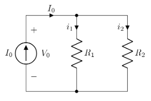
```tikz
\usepackage{circuitikz}
\begin{document}

\begin{circuitikz}[american, voltage shift=0.5]
\draw (0,0)
to[isource, l=$I_0$, v=$V_0$] (0,3)
to[short, -*, i=$I_0$] (2,3)
to[R=$R_1$, i>_=$i_1$] (2,0) -- (0,0);
\draw (2,3) -- (4,3)
to[R=$R_2$, i>_=$i_2$]
(4,0) to[short, -*] (2,0);
\end{circuitikz}

\end{document}
```

alt text

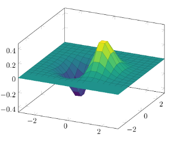
```tikz
\usepackage{pgfplots}
\pgfplotsset{compat=1.16}

\begin{document}

\begin{tikzpicture}
\begin{axis}[colormap/viridis]
\addplot3[
	surf,
	samples=18,
	domain=-3:3
]
{exp(-x^2-y^2)*x};
\end{axis}
\end{tikzpicture}

\end{document}
```

alt text

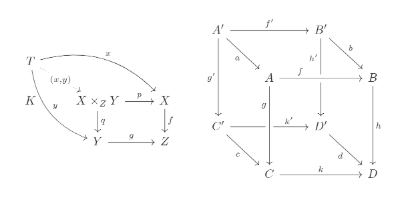
```tikz
\usepackage{tikz-cd}

\begin{document}
\begin{tikzcd}

    T
    \arrow[drr, bend left, "x"]
    \arrow[ddr, bend right, "y"]
    \arrow[dr, dotted, "{(x,y)}" description] & & \\
    K & X \times_Z Y \arrow[r, "p"] \arrow[d, "q"]
    & X \arrow[d, "f"] \\
    & Y \arrow[r, "g"]
    & Z

\end{tikzcd}

\quad \quad

\begin{tikzcd}[row sep=2.5em]

A' \arrow[rr,"f'"] \arrow[dr,swap,"a"] \arrow[dd,swap,"g'"] &&
  B' \arrow[dd,swap,"h'" near start] \arrow[dr,"b"] \\
& A \arrow[rr,crossing over,"f" near start] &&
  B \arrow[dd,"h"] \\
C' \arrow[rr,"k'" near end] \arrow[dr,swap,"c"] && D' \arrow[dr,swap,"d"] \\
& C \arrow[rr,"k"] \arrow[uu,<-,crossing over,"g" near end]&& D

\end{tikzcd}

\end{document}
```

alt text

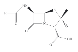
```tikz
\usepackage{chemfig}
\begin{document}

\chemfig{[:-90]HN(-[::-45](-[::-45]R)=[::+45]O)>[::+45]*4(-(=O)-N*5(-(<:(=[::-60]O)-[::+60]OH)-(<[::+0])(<:[::-108])-S>)--)}

\end{document}
```

alt text

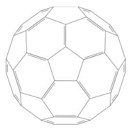
```tikz
\usepackage{chemfig}
\begin{document}

\definesubmol\fragment1{

    (-[:#1,0.85,,,draw=none]
    -[::126]-[::-54](=_#(2pt,2pt)[::180])
    -[::-70](-[::-56.2,1.07]=^#(2pt,2pt)[::180,1.07])
    -[::110,0.6](-[::-148,0.60](=^[::180,0.35])-[::-18,1.1])
    -[::50,1.1](-[::18,0.60]=_[::180,0.35])
    -[::50,0.6]
    -[::110])
    }

\chemfig{
!\fragment{18}
!\fragment{90}
!\fragment{162}
!\fragment{234}
!\fragment{306}
}

\end{document}
```

Where to generate tikz?

Geogebra (PC app)

File > Export > Graphics View as PGF/Tikz > Generate PGF/Tikz code > Copy everything except the first \documentclass line

Mathcha

Tutorial coming soon...

Latex examples

Useful tikz examples (math templates)

More tikz examples

Generic tikz examples

Where to generate tikz?

Geogebra (PC app)​

Mathcha​

Geogebra (PC app)

Mathcha